The HD Radio standard (NRSC-5) defines various “service modes,” which allow broadcasters to select how much bandwidth they would like to assign to their digital signal, and how that bandwidth should divided up. The standard defines many modes, but in practice almost all FM stations are using either:
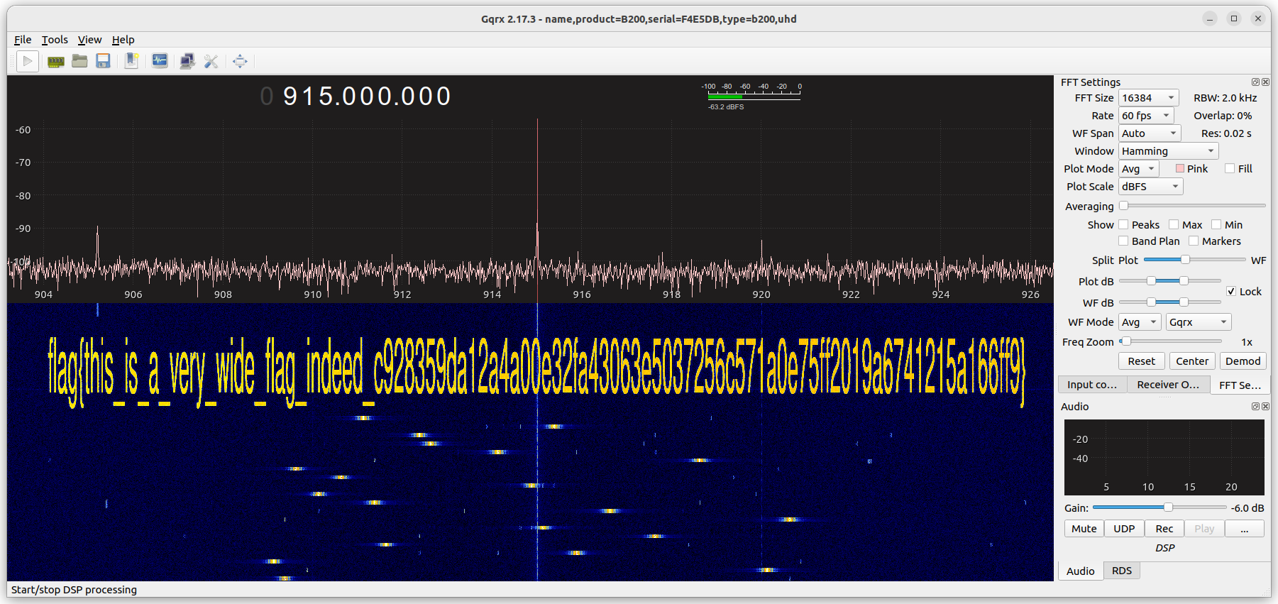
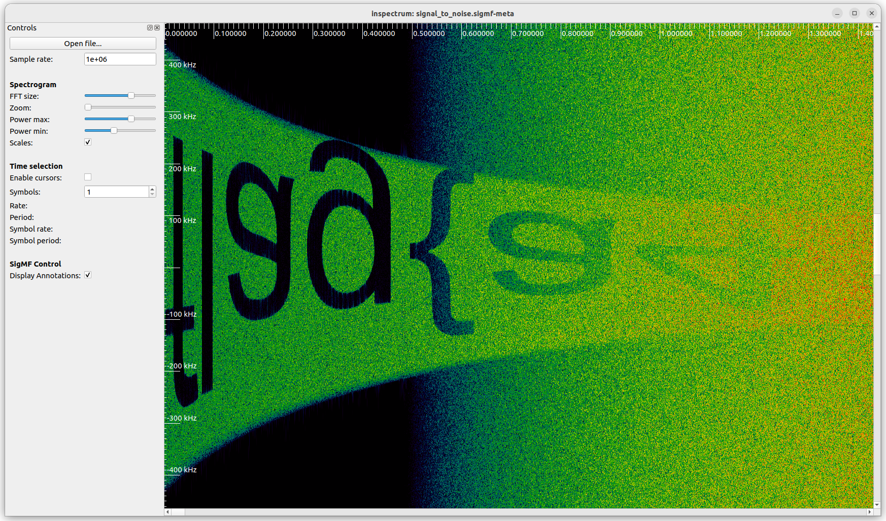
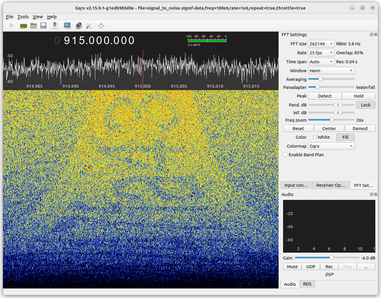
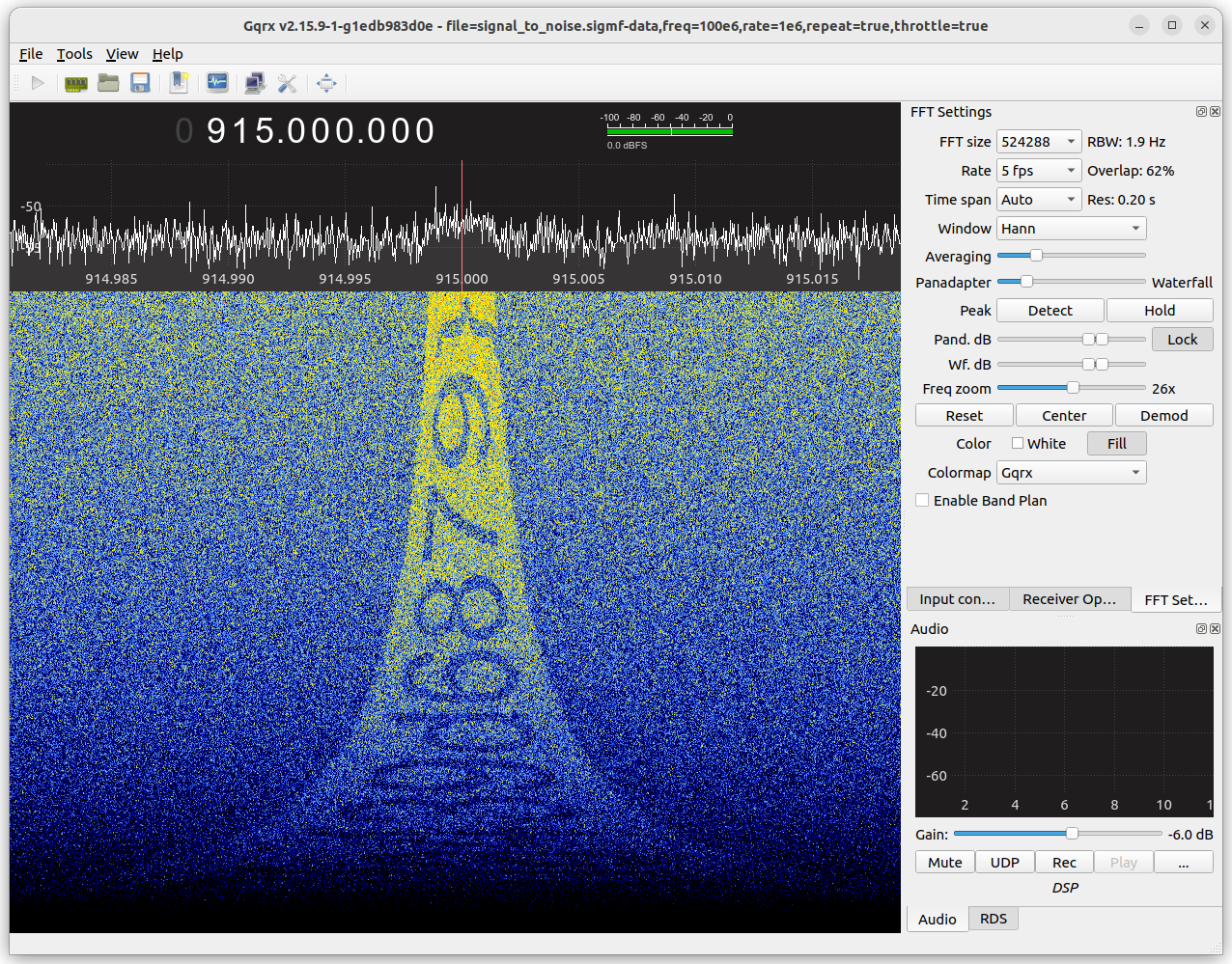
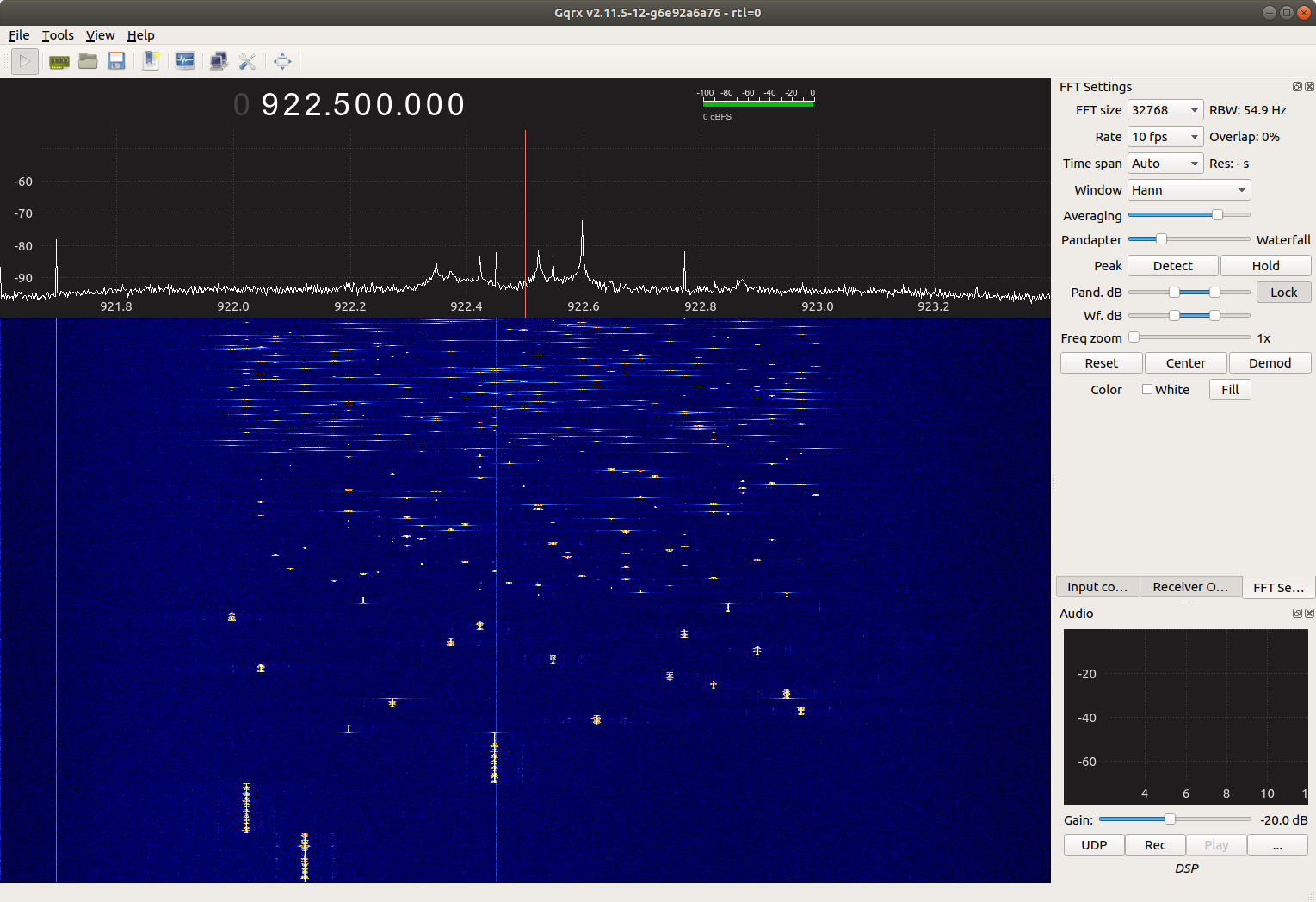
WWWT-FM recently began using MP11, which prompted me to look into this mode more deeply. It builds on top of MP3 by widening the digital signal further, increasing throughput to 149 kbit/s. Someone was kind enough to send me a recording of the WWWT-FM signal, but my trusty Sangean HDT-20 could not decode the additional subchannel. Nor could any of the other receivers we tried. A test signal generated by gr-nrsc5 didn’t work either, but I couldn’t be certain whether its MP11 implementation was correct.
After searching the web, I found a possible explanation in the Si468x Programming Guide:
Property 0x9A00. HD_SERVICE_MODE_CONTROL_MP11_ENABLE
This property Enables MP11 mode support. If MP11 support is disabled using this property the receiver will fall back to MP3 mode of operation when tuned to a station that is transmitting the MP11 subcarriers.
Default: 0x0000
Most HD Radio receivers use Si468x demodulator chips, and the Sangean HDT-20 is no exception. For reasons unknown, the chip does not decode the extra subchannel unless the receiver specifically opts in by switching on the HD_SERVICE_MODE_CONTROL_MP11_ENABLE
property. MP11 is the only service mode that gets this special treatment, so I can only speculate that perhaps a problem with an implementation of MP11 was discovered after it was standardized.
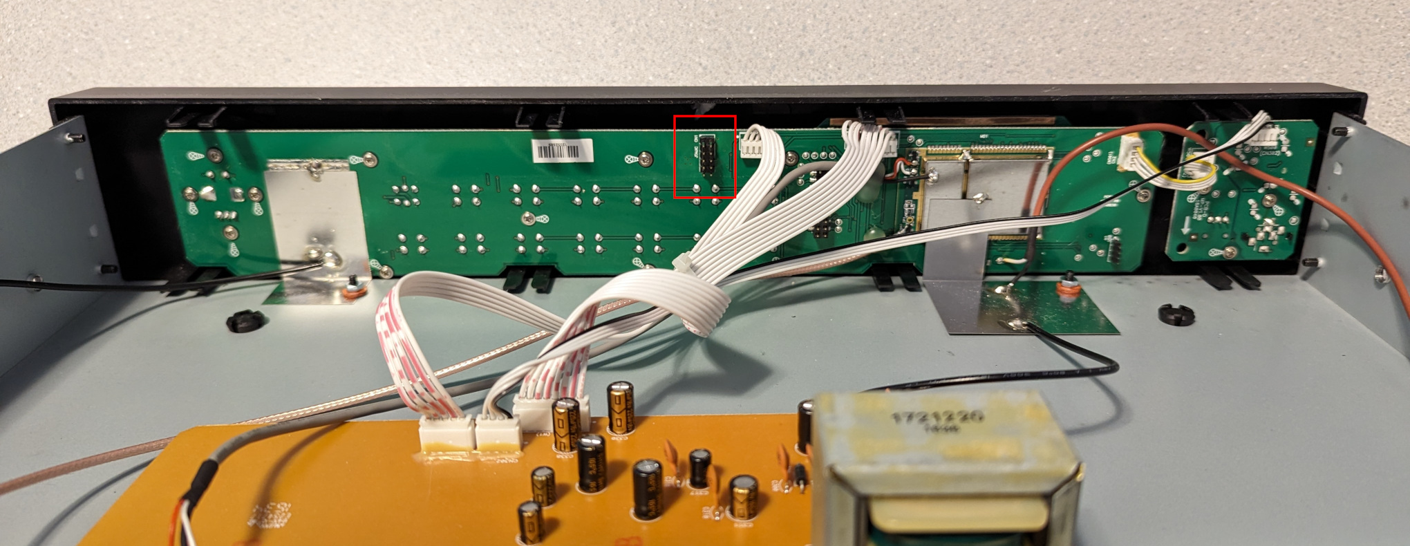
I wondered whether it might be possible to coax the HDT-20 into receiving MP11 by switching on the HD_SERVICE_MODE_CONTROL_MP11_ENABLE
property somehow. I opened up the receiver and found that the interesting bits were hidden inside an RF shield, but there was also a 10-pin header that looked suspiciously like a JTAG debug port.
I didn’t know much about JTAG, so I read over wrongbaud’s JTAG guide and installed JTAGenum on a Raspberry Pi to determine the JTAG pinout. It worked, and I was able to fetch the ID code register: 0x6974403f. This told me the manufacturer (0x01f = Atmel) and part number (0x9744). I made a few attempts to go further, but it became apparent that things would be difficult without using Atmel’s debugging hardware & software. So I bought an Atmel-ICE and installed Microchip Studio on a Windows machine.
I looked through Microchip Studio’s device definition files, and found that part number 0x9744 corresponds to the ATxmega192A3 and ATxmega192A3U microcontrollers. With that information in hand, I was able to probe the device and fetch its memory map:
C:\Users\Clayton\Documents>atprogram -t atmelice -i jtag -d ATxmega192A3 info
Firmware check OK
Tool atmelice has firmware version: 01.00
Target voltage: 3.20 V
Device information:
Name: ATxmega192A3
JtagId: 0x6974403f
Revision: G
CPU arch.: AVR8_XMEGA
Signature: 0x1e9744
Memory Information:
Address Space StartAddress Size
prog 0x0 0x32000
APP_SECTION 0x0 0x30000
APPTABLE_SECTION 0x2e000 0x2000
BOOT_SECTION 0x30000 0x2000
data 0x0 0x6000
IO 0x0 0x1000
MAPPED_EEPROM 0x1000 0x800
INTERNAL_SRAM 0x2000 0x4000
eeprom 0x0 0x800
signatures 0x0 0x3
fuses 0x0 0x6
lockbits 0x0 0x1
user_signatures 0x0 0x200
prod_signatures 0x0 0x34
FUSEBYTE5 (0b11100101 <-> 0xe5):
BODACT 0x2
EESAVE 0
BODLEVEL 0x5
FUSEBYTE4 (0b11110010 <-> 0xf2):
RSTDISBL 1
STARTUPTIME 0x0
WDLOCK 1
JTAGEN 0
FUSEBYTE2 (0b11111110 <-> 0xfe):
BOOTRST 1
BODPD 0x2
FUSEBYTE1 (0b00000000 <-> 0x00):
WDWPER 0x0
WDPER 0x0
FUSEBYTE0 (0b11111111 <-> 0xff):
JTAGUSERID 0xff
LOCKBITS (0b11111111 <-> 0xff):
BLBB 0x3
BLBA 0x3
BLBAT 0x3
LB 0x3
And then extract the firmware:
C:\Users\Clayton\Documents>atprogram -t atmelice -i jtag -d ATxmega192A3 read -fl -o 0x0 -s 0x30000 --format bin -f app_section.bin
Firmware check OK
Output written to app_section.bin
Back on my Linux machine, I was able to convert the firmware dump to ELF and disassemble it:
avr-objcopy -I binary -O elf32-avr app_section.bin app_section.elf
avr-objdump -D app_section.elf > app_section.asm
Since the Si468x Programming Guide has a list of property numbers, I decided to pick a couple (FM_SEEK_BAND_BOTTOM
= 0x3100, and FM_SEEK_BAND_TOP
= 0x3101) and see whether I could find those numbers in the firmware. I eventually found this interesting code fragment:
1bfa8: 60 91 ea 3b lds r22, 0x3BEA 1bfac: 70 91 eb 3b lds r23, 0x3BEB 1bfb0: 80 e0 ldi r24, 0x00 1bfb2: 91 e3 ldi r25, 0x31 1bfb4: 0e 94 c5 88 call 0x1118a 1bfb8: 60 91 e6 3b lds r22, 0x3BE6 1bfbc: 70 91 e7 3b lds r23, 0x3BE7 1bfc0: 81 e0 ldi r24, 0x01 1bfc2: 91 e3 ldi r25, 0x31 1bfc4: 0e 94 c5 88 call 0x1118a 1bfc8: 60 91 e2 3b lds r22, 0x3BE2 1bfcc: 70 91 e3 3b lds r23, 0x3BE3 1bfd0: 82 e0 ldi r24, 0x02 1bfd2: 91 e3 ldi r25, 0x31 1bfd4: 0e 94 c5 88 call 0x1118a 1bfd8: 60 e0 ldi r22, 0x00 1bfda: 70 e0 ldi r23, 0x00 1bfdc: 81 e0 ldi r24, 0x01 1bfde: 95 e3 ldi r25, 0x35 1bfe0: 0e 94 c5 88 call 0x1118a
It appears that the function at offset 0x1118a sets a property on the Si468x chip, taking the property number from registers r25 & r24, and the value from registers r23 & r22. So this code sets not only FM_SEEK_BAND_BOTTOM
and FM_SEEK_BAND_TOP
, but also FM_SEEK_FREQUENCY_SPACING
(property 0x3102) and FM_SOFTMUTE_SNR_ATTENUATION
(property 0x3501).
Assuming this code runs at boot, it should be possible to modify the instructions that set FM_SOFTMUTE_SNR_ATTENUATION
to instead set HD_SERVICE_MODE_CONTROL_MP11_ENABLE
(0x9A00) to 0x0001. The modified instructions are:
1bfd8: 61 e0 ldi r22, 0x01
1bfda: 70 e0 ldi r23, 0x00
1bfdc: 80 e0 ldi r24, 0x00
1bfde: 9a e9 ldi r25, 0x9A
On my Windows machine, I wrote the new instructions into the firmware:
C:\Users\Clayton\Documents>atprogram -t atmelice -i jtag -d ATxmega192A3 write -fl -o 0x1bfd8 --values 61e070e080e09ae9
Firmware check OK
Write completed successfully.
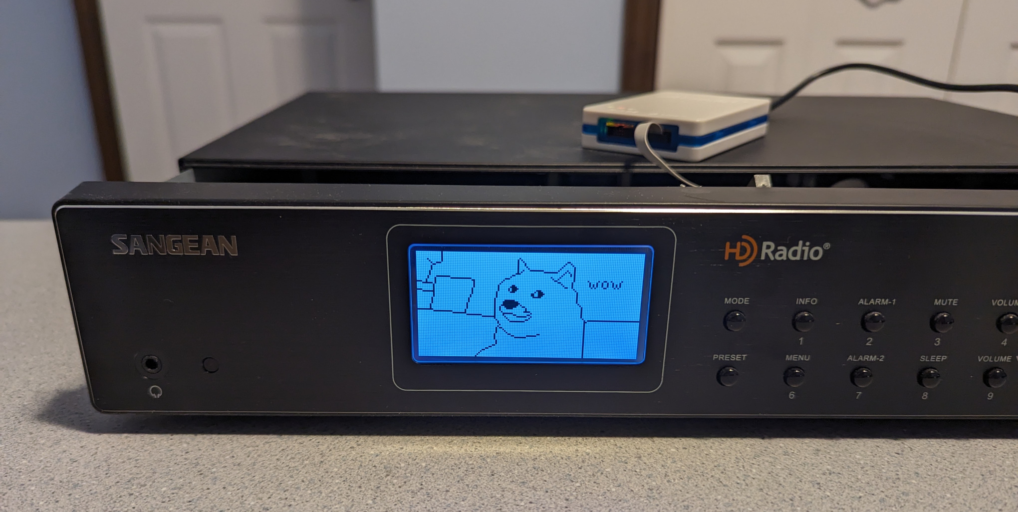
It worked! After rebooting the HDT-20, I was finally able to receive an MP11 signal.
While this patch worked, I was worried that failing to set the FM_SOFTMUTE_SNR_ATTENUATION
property might cause trouble, so I instead overwrote that code with a jump to an unused memory location:
1bfd8: 0d 94 00 78 jmp 0x2f000
At that location, I placed code to set both FM_SOFTMUTE_SNR_ATTENUATION
and HD_SERVICE_MODE_CONTROL_MP11_ENABLE
, then jump back:
2f000: 60 e0 ldi r22, 0x00
2f002: 70 e0 ldi r23, 0x00
2f004: 81 e0 ldi r24, 0x01
2f006: 95 e3 ldi r25, 0x35
2f008: 0e 94 c5 88 call 0x1118a
2f00c: 61 e0 ldi 22, 0x01
2f00e: 70 e0 ldi r23, 0x00
2f010: 80 e0 ldi r24, 0x00
2f012: 9a e9 ldi r25, 0x9A
2f014: 0e 94 c5 88 call 0x1118a
2f018: 0c 94 f2 df jmp 0x1bfe4
To write the patched code, I ran:
atprogram -t atmelice -i jtag -d ATxmega192A3 write -fl -o 0x1bfd8 --values 0d940078
atprogram -t atmelice -i jtag -d ATxmega192A3 write -fl -o 0x2f000 --values 60e070e081e095e30e94c58861e070e080e09ae90e94c5880c94f2df
If needed, the original code could be restored like so:
atprogram -t atmelice -i jtag -d ATxmega192A3 write -fl -o 0x1bfd8 --values 60e070e0
atprogram -t atmelice -i jtag -d ATxmega192A3 write -fl -o 0x2f000 --values ffffffffffffffffffffffffffffffffffffffffffffffffffffffff
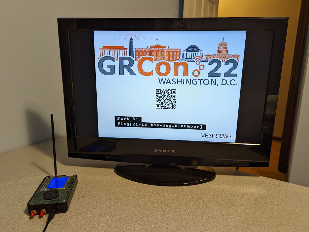
Now that I was comfortable modifying the firmware, I decided to have some fun with it. Why not change the bootup logo? After digging through the firmware dump, I found the bitmap at offset 0x1ca1 and was able to decode and display it with Python:
from PIL import Image
with open("app_section.bin", "rb") as f:
data = f.read()
offset = 0x1ca1
width, height = 128, 64
len_bytes = width * height // 8
image_data = data[offset:offset + len_bytes]
img = Image.new('1', (width, height))
for row in range(height // 8):
for col in range(width):
pixels = image_data[row*width + col]
for r in range(8):
img.putpixel((col, row*8 + r), (pixels >> (7-r)) & 1)
img.show()
With a bit more Python, I was able to convert my own image into the correct format:
from PIL import Image
img = Image.open("doge.png")
pix = img.load()
width, height = img.size
image_data = []
for row in range(height // 8):
for col in range(width):
pixels = 0
for r in range(8):
pixels |= ((1 if pix[col, row*8 + r][1] == 0 else 0) << (7-r))
image_data.append(pixels)
image_data = bytes(image_data)
print(image_data[:1024].hex())
And write the bytes to flash:
atprogram -t atmelice -i jtag -d ATxmega192A3 write -fl -o 0x1ca1 --values fffffffffffff7fbfdfefefdfdfd03fffffffffffffffffffffffffffffffffffffffffffffffffffffffffffffffffffffffffffffffffffff0eff7fbfcfffffffffffffffffffffffffffffffffffffffffffefdfbfbfdfefffffffffffffffffffffffffffffffffffffffffffffffffffffffffffffffffffffffffffffffffffffffffffce31ffffefdfdfdfdfdfdfdfdfefefefefefefefefefefefefffffffffffffffffffffffffffffffffffffffefefefdfbfbf707f7efdfff7fbfdfdfdfdfdfdfdfdfefefefefedeeefefdebd7bf7efdfeff3ff00ffffffffffffffffffffffffffffffffffffffffffffffffffffffffffffffffffffffffffffbdbdbddede1edededee01fffffffffffffffffffffffffffffffffffffffff7807fffffffffffffffffffffffffee1dfbf7ffffff9f6e0e0f1fbfffffffffffffffffffefdfcfcfeffffffffffff7f7fbfbfdfeff7f7ffff877bfdfeffffffffff7f8ff7cff78f7fff8f77778fff7f8ff7cff78f7ffffffffffffffffffffffffffffffffffffffee11ffffffffffffffffffffffffffffffffffffffce39f7fffffffffffffffffffffffffe01ffffffef8f0f0f0f0f0f0f8f8fdfeffffffffff3f1fdfdf1f1f3f7fffffffffffffffffffffffffffffffffffff03fdfeffffffffffffffffffffffffffffffffffffffffffffffffffffffffffffffffffffdfdfdfdfdfdfdf1fdfefefefefefefefefefefeff7f7f7f7f7f7f7c73bfbfbfbfbfbfbfbfbfdfdfdfdfdfdfd00ffff1feff375363737377b7bfdfdfd7d6d8debeaf5ffffffffffffffffffffffffffffffffffffffffffffffffffffffff01feffffffffffffffffffffffffffffffffffffffffffffffffffffffffffffffffffffffffffffffffffffffffffffffffffffffffffffffffffffffffffffffffffffffffffffffffffffffffff7897ebfbfdfeff7fbfbfbfbfbfbfbfbfbf7f7fffffffffffffffffffffffffffffffffffffffffffffffffffffffffffffffff00bf7f7f7f7f7f7f7f7f7f7f7f7f7f7f7f7f7f7f7f7f7f7f7f7f7f7f7f7f7f7fffffffffffffffffffffffffffffffffffffffffffffffffffffffffffffffffffffffffffffffffffffffff8778ffffffffff7fbfbfdfdfefefefefefefefdfdfdfdfdfdfbfbfffffffffffffffffffffffffffffffffffffffffffffffffff00fffffffffffffffffffffffffffffffffffffffffffffffffffffffffffffffffffffffffffffffffffffffffffffffffffffffffffffffffffffffffffffffffefdfbf7efefdfdfbfbf7f7fffffffffffffffffffffffffffffffffffffffffffffffffffffffffffffffffffffffffffffffffffffffffffffffffffffff00ffffffffffffffffffffffffffffffffffffffffffffffffffffffffffffff
Success!
]]>CTF players were asked to imagine they were employees of “Hackers 4 Cash,” a consulting firm hired by pickle farm “Ye Olde Pickles” to hack their competitor, “CyberPickle.” Not surprisingly, CyberPickle relied heavily on radio to automate their operations.
The first radio challenge was called “Wide Load,” and players were given the following challenge:
To keep their communications private, CyberPickle is testing out a new wideband communication system on the 902-928 MHz ISM band. Is it possible to intercept the message?
When tuning to the low end of the band, around 905 MHz, the following signal appeared in the waterfall once every 45 seconds:
Clearly that’s the start of a flag, but we need to tune higher to see more. After tuning to 907 MHz and patiently waiting, the next piece of the flag could be seen:
After repeating this process another nine times or so, players would finally reach the end of the flag:
Many players asked me whether it’s possible to “zoom out” and see more of the radio spectrum at once. Unfortunately, it’s not possible to do that directly because the RTL-SDR is limited to a sample rate of approximately 2.4 million samples per second, which means that it’s only possible to see a frequency span of 2.4 MHz at a time. (In practice, the usable bandwidth is a bit lower than that due to aliasing; if you look closely at the screenshots above, you’ll see that signals near the edges of the display begin fading out and then “wrap around” to the opposite edge due to the imperfect anti-aliasing filter in the receiver.)
More expensive receivers can operate at much higher sample rates. For instance, the USRP B200 can receive up to 56 MHz at once, allowing the entire 902-928 MHz ISM band to be recorded:
To create this challenge, I used ImageMagick to create a large PNG file containing the flag, and then painted that onto the radio spectrum using gr-paint. I’ve published the source code for all my challenges, and the pieces used to generate the “Wide Load” challenge can be found here and here.
]]>Photo by Simon Carpentier is licensed under CC BY-NC 4.0
I wanted to reverse engineer the badge-to-badge communication protocol, and soon found out that it was asynchronous serial at 38400 baud, but with inverted polarity. While my Saleae logic analyzer happily decoded the inverted signal, my Raspberry Pi Debug Probe could not. I worked around the problem by building a couple inverters (one for transmit, one for receive) on a breadboard, and putting them between the badge and the Debug Probe. This worked, but it was cumbersome enough that I wanted to find a better solution.
After searching the web and digging through datasheets, I learned that the RP2040 chip’s GPIO pins can be inverted by setting GPIO control registers (specifically, the INOVER
and OUTOVER
fields in the GPIO*_CTRL
registers). The gpio_set_outover
and gpio_set_inover
functions in the Raspberry Pi Pico SDK provide a convenient way to set these registers. It only took a couple lines of code to invert the UART pins in the Debug Probe firmware.
In case you’d like to try this out on your own Debug Probe, I’ve posted the compiled firmware on GitHub.
]]>The event was a phenomenal success. There were 52 challenges, and 71 teams submitted 686 valid flags. Even though the competition period has ended, most of the challenges are still up and playable at https://ctf-2022.gnuradio.org/.
In this post, I’ll describe how I created my challenges, and how I anticipated they might be solved. If you don’t want any spoilers, stop reading here!
This challenge track consisted of 13 flags embedded in 11 signals, all contained in a single SigMF recording. I expected that players might use the Signal Identification Wiki to help identify the signals and find decoding software.
From left to right, the signals were:
This challenge has its origins in a tutorial session I created for the Ottawa Amateur Radio Club in 2014. I later published the source code, and in 2019 I adapted it for use as a CTF challenge at BSides Ottawa. For GRCon22, I added M17, a promising open-source alterative to proprietary digital voice protocols.
Most of the signals can be received directly within Gqrx, but a few require additional software. To test the challenges, I used the following:
If you solved the SSTV challenge, you can also receive the SSTV images that the International Space Station occasionally broadcasts on 145.800 MHz!
This challenge was inspired by amateur radio direction finding (also known as radio fox hunting) where competitors run through the woods searching for hidden radio transmitters.
I built two hidden transmitters (“foxes”) which transmitted Morse code. One ran at approximately 433 MHz, and was hidden at a fixed location in the conference area. The other transmitted at approximately 904 MHz, and was carried around by various conference organizers in their backpacks, making it a moving target. Players had to determine the exact frequency of each transmitter, copy the flag which was included in the Morse code message, and then physically locate the transmitter to read another flag which was printed on it. Here’s a peek inside the hidden transmitters:
I built them with Adafruit Feather M0 RFM69HCW Packet Radios, which are available in 433 MHz and 915 MHz versions. These boards are normally used to transmit and receive FSK signals, but they also have an on-off keying mode where the transmitter can be switched on and off using a GPIO pin. That makes it easy to tap out a message in Morse code. Each transmitter is powered by a 2000 mAh lithium cell, which is enough to provide four days of power.
Gqrx does a fine job of receiving the Morse code, and it’s even possible to read it by eye from the waterfall:
Although directional antennas can be helpful to find hidden transmitters, most players got by with omnidirectional antennas. I recommend putting on a pair of headphones and disabling both hardware and software AGC, thus making the audio amplitude directly proportional to the incoming RF signal power. Walking closer to the transmitter will then make the signal louder, and walking away will make it quieter. Once you’re close enough to the signal that the receiver is saturated (and audio begins clipping), reduce the RF input gain and keep searching for a stronger signal. When you get very close and your RF gain is already at a minimum, it may be necessary to switch to a worse antenna or remove the antenna completely. Beware that some things other than distance from the transmitter also affect received signal power. For instance, obstacles may absorb or reflect radio signals.
In this challenge, the start of a spectrum-painted flag is apparent when the signal is viewed in inspectrum, but as time progresses the signal narrows in frequency, widens in time, and is engulfed by an ever-increasing amount of noise. By playing with the “FFT size”, “Power max”, and “Power min” settings it is possible to read off the first half of the flag: flag{a4146a8247
. But the remainder is impossibly difficult to read.
Fortunately, Gqrx allows larger FFT sizes and finer control over the FFT rate, which is just barely enough to read off the rest of the letters:
By stitching these parts together, we get the complete flag: flag{a4146a8247fa439d6879}
.
To make this challenge, I used gr-paint to generate a rectangular spectrum-painted image, then passed this through a Polyphase Arbitrary Resampler block with progressively increasing resampling rate, and added noise from a Gaussian noise source with progressively increasing amplitude. A Python script dynamically adjusts the parameters of the resampler and noise source after each line from the rectangular image is processed.
The name of this challenge hints at NTSC, an analog television standard. Engineers jokingly referred to it as “Never The Same Color” because its colour accuracy was sometimes poor.
The challenge consisted of an NTSC signal containing seven flags. One was in the video, four were in the audio (mono, stereo, second audio program, and PRO subcarrier), and two were in EIA-608 closed captions (channels CC1 and CC3). One twist was that the video flag only appeared once every 176 frames. The other frames contained a decoy. (If you’re curious, scan the QR code in the image below to see what it was!)
To produce the signal, I made some improvements to the NTSC signal generator from my SDR examples repository, and tested with a television set. In fact, every flag except for the PRO (professional) subcarrier can be received by an ordinary television set:
Many players found the flags this way, piping the signal into a nearby television. (Even the television sets in guest rooms at the conference hotel could be coaxed into receiving NTSC.) But I was very impressed by Daniel Estévez, who built his own NTSC demodulator in a Jupyter notebook!
This was my favourite challenge, and I had a lot of fun building it.
The challenge description asked the player to transmit an APRS packet at 903.5 MHz, with their team name as the source address and “new” in the comment field. A response would then arrive somewhere in the 900 MHz ISM band. In fact, it arrived at 926 MHz in the form of a spectrum-painted rules page for a variation of Wordle called “SDRdle”:
All the player had to do at this point was follow the instructions and transmit further APRS packets containing their guesses:
To test the challenge, I used Dire Wolf to generate APRS packets and place them in WAV files:
echo "ARGILO>WORLD:>new" | gen_packets -r 48000 -o aprs.wav -
I then made a simple flow graph to FM-modulate them and transmit them on a HackRF.
The challenge server received APRS packets using rtl_fm piped into Dire Wolf, generated game board images using the Python Imaging Library, and transmitted them using gr-paint.
Source code for all of the above challenges can be found in my grcon22 GitHub repository. I’ve released the code under the GPL so that they can be adapted and used for other purposes. If you use them for an event of your own, I’d love to hear about it!
I hope players had as much fun solving the challenges as I did creating them.
]]>When players tuned to 922.125 MHz, they were greeted with a narrow-band FM signal: “This is VE3IRR. The first flag is tango…” And then the signal hopped down to 922.025 MHz. Tuning there would reveal some more letters of the flag: “…victor echo uniform golf whiskey tango papa papa…” Next the signal hopped up to 922.450 MHz, providing the end of the flag: “…kilo sierra hotel delta victor tango charlie.” Of course, you’d invariably miss some of the letters while tuning from one frequency to the next. But since the signal repeated about once per minute, you could camp out on any one of the three frequencies and wait for the piece you were missing to be transmitted again. Players were awarded with 50 points for putting together the three pieces.
Then the problem got harder. Part two (worth 100 points) was similar, except that the signal hopped once per second. This challenge could be completed in a similar fashion, as long as you had a lot of patience. Part three (worth 150 points) had 5 hops per second, and part four (worth 200 points) had 50 hops per second! Clearly these were too hard to be solved by hand, and so a better approach was needed.
Here’s how things looked on the waterfall, with part one at the bottom and part four at the top:
There are several ways to approach this problem, but the end goal is always the same: to remove the hopping component from the signal so the audio can be demodulated.
My favourite approach is to take advantage of aliasing. Usually aliasing is a bad thing, because it causes two or more input frequencies to map to the same output frequency, making them indistinguishable. But in the case of a frequency hopping signal, it would actually be helpful if all the channel frequencies were mapped into a single one! To make this happen, all we need to do is sample the signal at some integer multiple of the channel spacing, then downsample the signal by keeping one out of every n samples, where n is the ratio of the sample rate to the channel spacing.
In this case, the channel spacing is 25 kHz, so we can sample the signal at 2 MHz and keep one out of every 2,000,000 / 25,000 = 80 samples. GNU Radio provides a “Keep 1 in N” block to do exactly that. We can then increase the sample rate back to a more convenient 96,000 samples per second and run it through an FM demodulator:
One disadvantage of this approach is that the noise in all the channels is combined. But as long as the signal-to-noise ratio is high and only a single channel is transmitting at a time, that’s not a problem. This receiver works beautifully, and all the flags can easily be heard.
Another approach is to demodulate the entire band as if it was a single FM signal. This will result in a step function being added into the audio signal. Since this step function is mostly a DC signal, we can remove it with a DC Blocker (a special type of high-pass filter):
This mostly works, but a noisy “pop” bleeds through the filter every time a hop occurs. In part four this results in a loud buzz at 50 Hz, but the flag can still be heard.
A third approach, which a friend of mine came up with during the competition, is to use a fast Fourier transform to detect which channel is active, and use that information to shift the input signal up or down in frequency so as to map the active channel’s frequency to zero. Here I’ve used an Argmax block to detect which FFT bin contains the most energy, a VCO (voltage controlled oscillator) block to generate a signal whose frequency is the negative of the active channel’s offset, and a Multiply block to combine the VCO with the input signal, shifting the frequency up or down as required:
This flow graph provides a very clean output signal, and would work well even if the signal-to-noise ratio was lower.
In case you’re curious, here’s the GNU Radio flowgraph I used to create sample files for each of the four parts of the challenge. The Vector Source and Repeat blocks generate a random step function, and the VCO and Multiply blocks shift the FM signal up or down in frequency in proportion to the step function.
In the end, 16 teams solved part one, four got part two, and two teams got all four parts.
]]>My favourite radio challenge was called “Waterfall”. When players tuned to 924.5 MHz, they saw the BSides Ottawa logo painted onto the waterfall, followed by the start of a flag:
At this point it seemed as though you just had to patiently wait for the rest of the flag to scroll by. But as time went on, the letters in the flag got smaller, and smaller, and smaller:
By the end, the letters were much too small to read in Gqrx, even when the FFT rate was increased to the maximum of 60 fps!
Fortunately, there are other tools which are designed for offline signal analysis, and which allow the user to have a much closer look at short, bursty signals. My favourites are Inspectrum and Baudline. After capturing the signal to a file with Gqrx’s “Record and play I/Q data” button, it was easy to read off the tail end of the flag with Baudline:
So how did I build this challenge? I needed two things: a way to distort an image so it would become thinner and thinner at one end, and a way to paint that image onto the radio spectrum.
To produce the distorted image, I used ImageMagick’s FX special effects image operator, which allows the user to define an arbitrary mapping between input pixels and output pixels. After some experimentation, I found that transforming the y axis using an exponential function worked best:
convert \
\( \
-background White \
-gravity Center \
-pointsize 400 \
label:flag\{look_closer_a4146a8247fa439d6879\} \
-rotate 270 \
\) \
bsides-ottawa-logo.jpg \
-append \
-crop 50x100%-30+0 \
-gravity North \
-extent 100%x200% \
-fx "xx = i; yy = ln(j/7978/2 * (exp(5)-1) + 1) / 5 * 7978; v.p{xx,yy}" \
logo-flag.png
Painting the resulting image onto the spectrum was easy, thanks to gr-paint, a GNU Radio module written by Ron Economos (a.k.a. @drmpeg). This module takes an image file as input, and uses an inverse FFT to map each row of pixels into a set of OFDM carriers with the corresponding amplitudes.
It was a joy to watch players copying down the start of the flag, only to realize they would have to work harder to get the rest. The first person to solve the problem was my friend and former colleague Serge Mister from Entrust Datacard’s “Reverse Solidus” team. By the end of the competition, another 12 teams had solved it.
]]>I was already aware that Ottawa’s water meters use the ERT protocol, which can be received using an RTL-SDR dongle and rtlamr. I installed the program on an old laptop, and stored its output in a file with rtlamr | tee usage.txt
. I checked my meter number and ran tail -f usage.txt | grep 12345678
to confirm I was receiving packets from it. Fresh packets were arriving every few minutes. After a few hours it became apparent that the resolution of the readings was 0.05 m³, and that the reading only changes once per hour, on the hour.
With this information in hand, I put together a Python script to extract my meter’s readings from the file, keep the first reading from each hour, and plot the results with Pyplot:
#!/usr/bin/env python3
import matplotlib.pyplot as plt
import dateutil.parser
import re
MY_ID = 12345678
regex = re.compile(r"{Time:(.*) SCM:{ID:\s*(\d*) .* Consumption:\s*(\d*) .*")
times = []
usages = []
last_time = None
for line in open('usage.txt'):
result = regex.match(line)
if not result:
print("Error parsing line:")
print(line)
exit(1)
id = int(result[2])
if id != MY_ID:
continue
time = dateutil.parser.parse(result[1])
measurement_time = time.replace(minute=0, second=0, microsecond=0)
consumption = int(result[3]) / 100
if measurement_time != last_time:
times.append(measurement_time)
usages.append(consumption)
last_time = measurement_time
plt.figure(figsize=(14, 9))
plt.plot(times, usages)
plt.grid(True)
plt.show()
Here’s the result after a week collecting packets:
During the first few days, I observed that water was consumed at about 0.05 m³ every five hours even when I was away from home, suggesting that the leak was about 10 litres per hour. I turned off the input values to my toilets, and the next day the reading stayed constant all day. The flappers in two of the toilets had warped with age, and replacing them brought water consumption back to normal.
Of course, I could have just run down to the basement now and then to read the meter, but where would the fun be in that?
]]>The first step was to figure out what frequency the controller was transmitting on. The BladeRF makes that a fairly easy task, since it has a bandwidth of 28 MHz. I fired up gqrx to get a nice waterfall view of all that bandwidth. My first guess was that the signal might be on the 902-928 MHz band, and sure enough, I spotted a signal popping up at 911.24 MHz whenever I pressed a button on the controller. But it was quite weak, which led me to suspect it might be a harmonic. Indeed, when I tuned lower I found a very strong signal at 303.747 MHz, and I could easily detect it from across the room.
The next step was to check what modulation scheme the controller used. Most simple devices like this are using either on-off keying or frequency-shift keying. Zooming in on the signal in gqrx, I saw only a single peak, which suggested on-off keying.
I knew my trusty RTL-SDR dongle would be more than capable of receiving and demodulating the signal, so I threw together a very simple GNU Radio flow graph to show me the amplitude of the 303.747 MHz signal over time:
Here’s what I saw on the scope, once I set it to trigger on a rising edge and pressed the “light” button on the ceiling fan controller:
The transmission was short enough that I could just read the bits off visually: 1011011001011001001001001001001001011. And by measuring the time from the start to the end of those bits, I worked out that the symbol rate was about 3211 baud.
In fact, all the buttons generated very similar 37-bit patterns:
off: 1011011001011001001001001001001011001
low: 1011011001011001001001001011001001001
med: 1011011001011001001001011001001001001
high: 1011011001011001001011001001001001001
light: 1011011001011001001001001001001001011
The bits were repeated for as long as a button was held, with about another 37 bits worth of zeroes between each repetition.
Given this information, it was trivial to build a flow graph to transmit an on-off keying signal using the BladeRF:
My first attempt was unsuccessful, but it turned out the problem was just that the output gain wasn’t set high enough. Bringing it up to about 15 dB was sufficient to reliably control the ceiling fan!
The whole reverse engineering project took only about a half an hour, which really demonstrates the power of software-defined radio.
I’ve already added the receiver and transmitter to my sdr-examples repository on Github:
Receiver: ceiling_fan_rx.grc
Transmitter: ceiling_fan_tx.grc
Update: Looking at the bit patterns above, it is apparent that the bits come in groups of three: either 001 or 011. Presumably, 001 represents a baseband 0, and 011 represents a baseband 1. That is, a narrow pulse represents a zero and a wide pulse represents a one. That would make the baseband bit patterns as follows:
off: 0110100000010
low: 0110100001000
med: 0110100010000
high: 0110100100000
light: 0110100000001
First off, you’ll need two laptops running Linux: one to transmit, and one to receive. The transmit laptop needs to have the latest version of GNU Radio installed. If you’re running Ubuntu, the easiest way to get that done is to use OZ9AEC’s package archive. At a command prompt, run the following:
sudo add-apt-repository ppa:gqrx/snapshots
sudo apt-get install gnuradio gnuradio-dev gqrx libboost-all-dev libcppunit-dev swig liblog4cpp5-dev
Once that’s done, you’ll need to install YO3IIU’s DVB-T package for GNU Radio:
git clone https://github.com/BogdanDIA/gr-dvbt.git
cd gr-dvbt
mkdir build
cd build
cmake -DCMAKE_INSTALL_PREFIX=/usr ../
make
sudo make install
sudo ldconfig
cd ..
Next, grab my collection of SDR examples:
git clone https://github.com/argilo/sdr-examples.git
Included in that collection is dvbt-blade.py, a script written by W6RZ that lets you transmit DVB-T from the command line using a BladeRF. Since amateur stations typically operate at much lower power than commercial broadcasters, I’ve modified it to use the lowest available bit rate, which should maximize the distance at which the signal can be received. (If you want to experiment with higher bit rates, you can change the “channel_mhz”, “mode”, “code_rate”, “constellation” and “guard_interval” variables. You’ll also need to adjust the mux rate of your transport stream, which can be calculated using W6RZ’s dvbrate.c.) The script is configured to transmit at a centre frequency of 441 MHz, so be sure to attach a suitable 70cm antenna to your BladeRF’s TX port before transmitting.
The script expects to be given an MPEG transport stream as input. Fortunately, we can produce one in real time using avconv. It can record video from the laptop’s webcam and audio from the laptop’s microphone, and encode them into a suitable transport stream. To let avconv and dvbt-blade.py talk to each other, we’ll create a fifo:
mkfifo in.fifo
Then we launch dvbt-blade.py and tell it to read from the fifo:
sdr-examples/dvbt-blade.py in.fifo
You’ll see some output, but nothing will be transmitted yet because no data is arriving in the fifo. To fix that, open a second terminal window and run avconv like so. Be sure to replace XXXXXX with your own call sign, which will be displayed in the lower right corner of the video.
avconv -f alsa -i pulse -f video4linux2 -s 640x480 -i /dev/video0 -vf drawtext=fontfile=/usr/share/fonts/truetype/freefont/FreeSerif.ttf:text="XXXXXX":x=440:y=420:fontsize=48:fontcolor=white@0.6:box=1:boxcolor=black@0.2 -vcodec mpeg2video -s 640x480 -r 60 -b 4000000 -acodec mp2 -ar 48000 -ab 192000 -ac 2 -muxrate 4524064 -mpegts_transport_stream_id 1025 -mpegts_service_id 1 -mpegts_pmt_start_pid 0x1020 -mpegts_start_pid 0x0121 -f mpegts -y in.fifo
You may need to install additional packages so that avconv has access to all the codecs it needs. If all goes well, your two terminal windows should look like this:
Now, over to the receiving laptop, which will use an RTL-SDR dongle to pick up the signal. Since support for the RTL2832 chip was only recently added to the Linux kernel, you’ll want to be running a recent Linux distribution such as Ubuntu 13.10. Make sure you have vlc installed:
sudo apt-get install vlc
Then launch vlc like so:
vlc dvb://frequency=441000000:bandwidth=6
If all goes well, you’ll see your video and hear your audio!
Now that you’ve succeeded on the 70cm band, you may want to try this on the 33cm and 23cm bands as well. Unfortunately, the Linux drivers for the RTL-SDR dongle currently limit its maximum frequency to 862 MHz, a bit below the 33cm band. Until the drivers get updated (I’ve already submitted a patch request), you can work around the problem by patching the kernel modules on your receiving laptop using the dvb-freq-fix.py script in my sdr-examples repository:
sudo sdr-examples/dvb-freq-fix.py
If everything worked correctly, the script should print out “Success!” twice. If you saw that, then reboot, and you should now be able to tune all the way up to 1750 MHz. On the transmitting laptop, change the “center_freq” variable to 913000000 for 33cm or 1279000000 for 23cm, put an appropriate antenna on your BladeRF’s TX port, and fire up dvbt-blade.py and avconv again. On the receiving laptop, fire up vlc again, putting the appropriate value in for the “frequency” parameter.
In my experiments, I found that the BladeRF put out the most power on the 33cm band. I was able to receive the signal all around the house, using a rubber duck 33cm antenna on the BladeRF and the RTL-SDR dongle’s stock antenna. I’ve had a QSO with VA3DGN on 70cm. To get the signal beyond my house, I hooked the BladeRF up to a Down East Microwave 70cm 25 watt power amplifier.
Have fun with DVB-T! I’d love to hear back if you make any contacts.
]]>Back in February, Linux kernel developer Antti Palosaari discovered that certain USB TV tuners can be configured to send the raw, unprocessed radio signal straight to the computer for decoding in software. (They use this mode when tuning FM or DAB radio signals. Think of it as the Winmodem approach to radio.) Palosaari realized that by running the right software, almost any radio signal could be received by these tuners. Not long thereafter, the RTL-SDR project was born, allowing these tuners to be used in Linux.
I should note that receiving (and transmitting) radio signals in software is nothing new. Software-defined radio has been around for years, but the hardware required (such as the Ettus Research USRP has generally been expensive. The availability of a $20 software-defined radio receiver has truly opened up the world of radio to anyone who takes the time to learn.
Since getting my hands on a compatible TV tuner, I’ve been able to listen to police radio, pager networks, garage door openers, air traffic control, and lots more. I recently tweeted that I had succeeded in tracking the aircraft in my area by using my TV tuner as an ADS-B receiver and feeding the output into Google Earth. This caught the interest of a pilot friend of mine, so I thought I’d put together a tutorial for anyone interested in capturing these signals. Although the tutorial is specific to ADS-B, keep in mind that the software tools (and in particular GNU Radio) can be reconfigured to tune in virtually any radio signal.
So let’s get started!
cd ~
mkdir build-gnuradio
cd build-gnuradio/
wget http://www.sbrac.org/files/build-gnuradio
chmod a+x ./build-gnuradio
./build-gnuradio
Note that GNU Radio is quite a large piece of software and has a lot of dependencies, so the install process can take a long time.
cd ~
git clone https://github.com/bistromath/gr-air-modes.git
cd gr-air-modes
cmake .
make
sudo make install
sudo ldconfig
uhd_modes.py --rtlsdr
If it works, you should see output like the following:
(-42 0.0000000000) Type 11 (all call reply) from c0636c in reply to interrogator 0 with capability level 6
(-41 0.0000000000) Type 17 BDS0,5 (position report) from c078b2 at (45.199942, -75.541590) at 30050ft
(-39 0.0000000000) Type 11 (all call reply) from c078b2 in reply to interrogator 0 with capability level 6
(-39 0.0000000000) Type 17 BDS0,9-1 (track report) from c078b2 with velocity 443kt heading 259 VS 1664
(-40 0.0000000000) Type 17 BDS0,5 (position report) from c078b2 at (45.199616, -75.544069) at 30075ft
(-42 0.0000000000) Type 17 BDS0,5 (position report) from c078b2 at (45.199265, -75.546504) at 30100ft
We’re already seeing some GPS coordinates and altitudes! Press CTRL-C to stop it for now. If you don’t see any traffic, try going outside for better reception.
xfonts-75dpi
and xfonts-100dpi
packages by running the following in a terminal window:
sudo apt-get install xfonts-75dpi xfonts-100dpi
Then log out and log back in so the new fonts will get loaded.
sudo ln -s /usr/lib/i386-linux-gnu/mesa/libGL.so.1.2 /usr/lib/libGL.so.1
uhd_modes.py
again, this time telling it to write its output to a KML file, the format used by Google Earth. In a terminal window, run the following:
uhd_modes.py --rtlsdr --kml=planes.kml
I hope you find this tutorial useful, and that you’ll do more exploring with software-defined radio once you’ve succeeded in watching planes!
]]>